Table of Contents
- 1 DeconvTest: simulation framework for quantifying errors and selecting optimal parameters of image deconvolution
- 2 Simulation of microscopy experiments
- 3 Reconstructing synthetic data with different deconvolution approaches
- 4 Quantification of deconvolution performance
- 5 Running DeconvTest in a batch mode
- 6 Running in silico deconvolution experiments with the "run_simulation" script
- 7 Deconvolving microscopy images with the help of DeconvTest
DeconvTest: simulation framework for quantifying errors and selecting optimal parameters of image deconvolution
![]()
Author: Anna Medyukhina
Affiliation: Research Group Applied Systems Biology - Head: Prof. Dr. Marc Thilo Figge
https://www.leibniz-hki.de/en/applied-systems-biology.html
HKI-Center for Systems Biology of Infection
Leibniz Institute for Natural Product Research and Infection Biology -
Hans Knöll Insitute (HKI)
Adolf-Reichwein-Straße 23, 07745 Jena, Germany
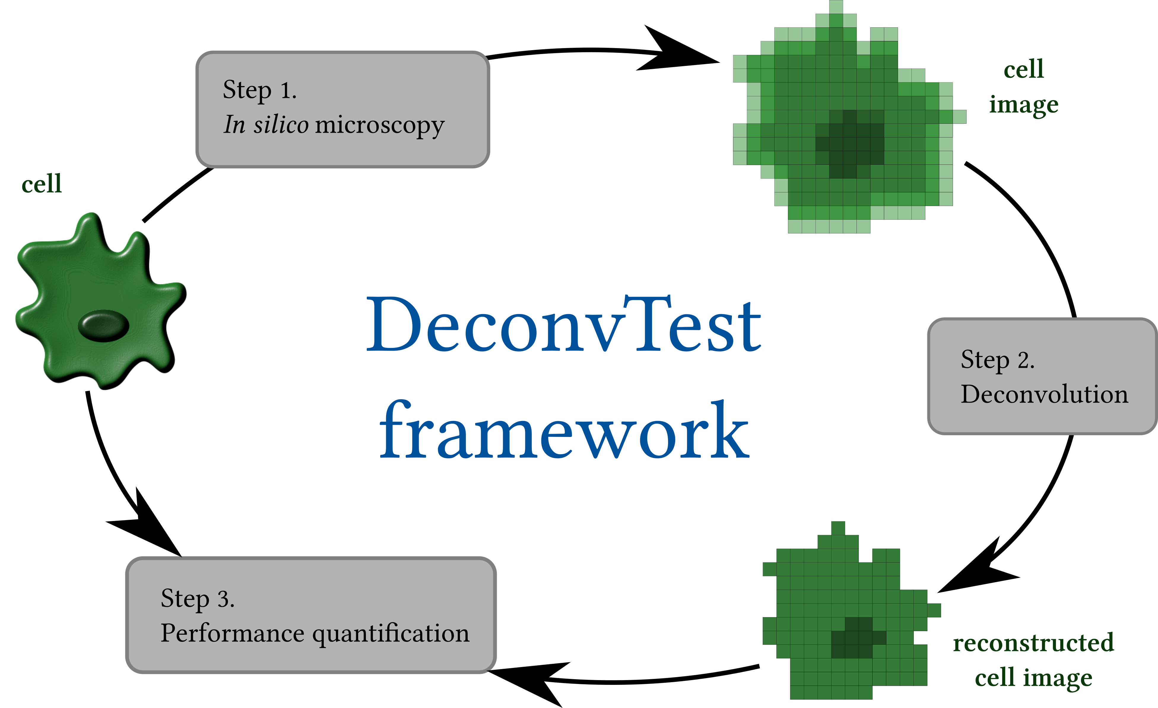
DeconvTest is a Python-based simulation framework that allows the user to quantify and compare the performance of different deconvolution methods. The framework integrates all components needed for such quantitative comparison and consists of three main modules: (1) in silico microscopy, (2) deconvolution, and (3) performance quantification.
Source code
The source code of the package can be found at https://github.com/applied-systems-biology/DeconvTest
Installation
- Download Fiji, make sure that the Fiji installation path does not contain spaces; note the Fiji installation path: you will have to provide it later when installing the DeconvTest packge
- Download the DeconvolutionLab_2.jar and Iterative_Deconvolve_3D.class and copy them to the plugins folder of Fiji
- Install python or python Anaconda
- Download the DeconvTest package, enter the package directory and install the package by running
python setup.py install - Provide the path to Fiji when prompted
Requirements
The software was tested with the following versions of the required packakges:
- scikit-image 0.15.0
- pandas 0.25.1
- numpy 1.16.5
- seaborn 0.9.0
- scipy 1.3.1
- ddt 1.2.1
License
The source code of this framework is released under the 3-clause BSD license
Simulation of microscopy experiments
Microscopic imaging of a sample involves illuminating the sample with a light source, collecting the emitted light, and discretizing the signal by recoding it in a detector, such as a CCD camera. This process can be represented as a continuous convolution of the sample with a point spread function (PSF) - the image of a point source - and subsequent discretization. Convolution of complex continuous signals is non-trivial to compute. Hence, when simulating this process on a computer, we represent the continuous convolution process by a convolution of discrete signals of high resolution (very small voxel size), while the process of discretization is simulated by the subsequent downsampling (decrease of the resolution).
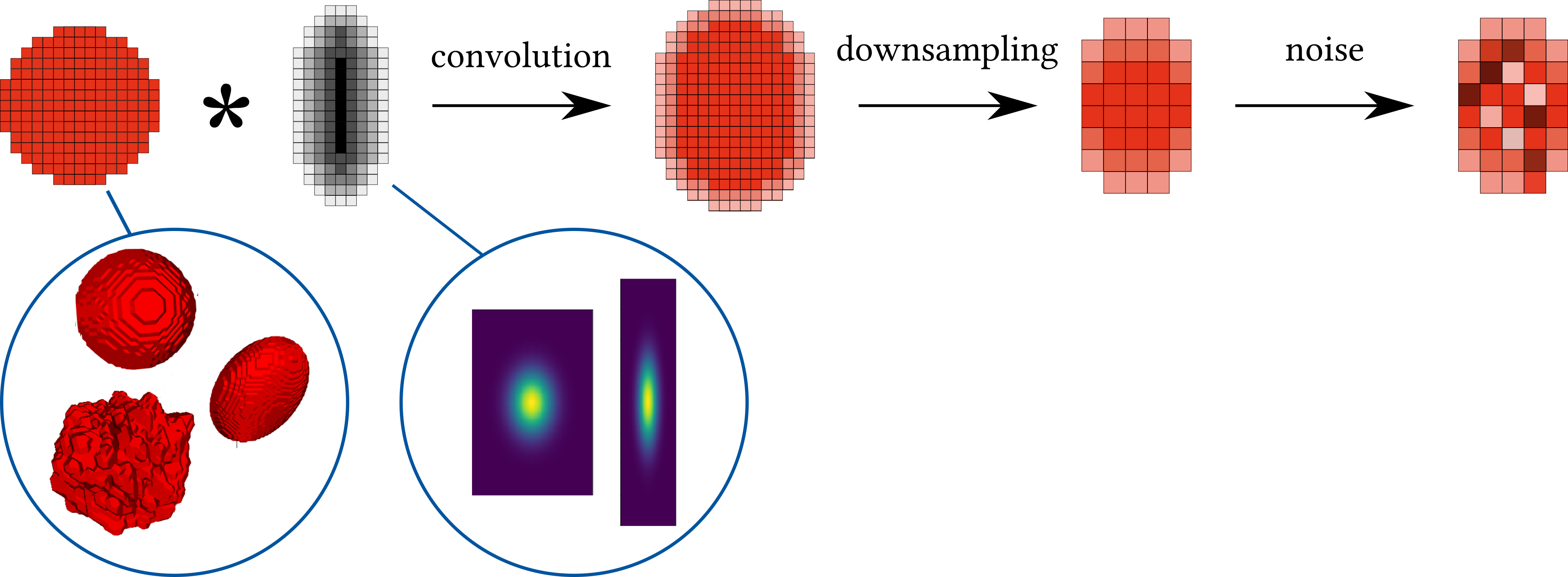
To simulate the whole microscopy process, we need to model the following steps and components:
- Images of cells
- Point spread function (PSF) of the imaging system
- Convolution and downsampling
- Noise
Generating synthetic cells
Synthetic cells can be generated with the class Cell, which is initialized with the following parameters:
from DeconvTest import Cell
print(Cell.__init__.__doc__)
Cell of ellipsoidal, as well as realistic shapes can be generated:
print(Cell.generate.__doc__)
cell = Cell(input_voxel_size=0.3,
            input_cell_kind='ellipsoid',
            size=10)
cell.show_2d_projections()

The input_cell_kind argument can be ommited in this case, because its default value is ellipsoid:
cell = Cell(input_voxel_size=0.3,
            size=10)
cell.show_2d_projections()
Example 2
Generate a cell with ellipsoidal shape with axes 10, 7, and 7 µm and voxel size 0.3 µm per px:
cell = Cell(input_voxel_size=0.3,
            size=[10, 7, 7])
cell.show_2d_projections()

Visualize the cell in 3D using ipyvolume:
import ipyvolume.pylab as p3
from IPython.core.display import HTML
p3.clear()
p3.plot_isosurface(cell.image)
p3.show()
Example 3
Generate a cell with ellipsoidal shape with axes 10, 7, and 7 µm and rotation of π/4 along the polar axis and π/2 along the azimuthal axis. Voxel size is 0.3 µm per px:
import numpy as np
cell = Cell(input_voxel_size=0.3,
            size=[10, 7, 7],
            phi=np.pi/4,
            theta=np.pi/2)
cell.show_2d_projections()

The cell sizes can be alternatively specified by the arguments size_x, size_y and size_z:
cell = Cell(input_voxel_size=0.3,
            size_x=7,
            size_y=7,
            size_z=10,
            phi=np.pi/4,
            theta=np.pi/2)
cell.show_2d_projections()
Example 4
Generate a spiky cell with spikiness 0.5 (i.e., 50% of cell surface covered by spikes), spike size 1 cell radius, and spike smoothness 0.05 (i.e., the size of the smoothing filter equals to 5% of cell radius); the cell has ellipsoidal shape with axes 10, 7, and 7 µm and rotation of π/4 along the polar axis and π/2 along the azimuthal axis; voxel size is 0.3 µm per px:
cell = Cell(input_cell_kind='spiky_cell',
            input_voxel_size=0.3,
            size_x=7,
            size_y=7,
            size_z=10,
            phi=np.pi/4,
            theta=np.pi/2,
            spikiness=0.5,
            spike_size=1,
            spike_smoothness=0.05)
cell.show_2d_projections()
p3.clear()
p3.plot_isosurface(cell.image)
p3.show()

Generating multicellular samples
To generate a multicellular sample one has to specify cell parameters (e.g. size and rotation) for each cell in the sample. This is done in two steps:
- Cell parameters for each sample are specified as
pandas.DataFrame, or as an instance of the classCellParams, where the cell parameters are generated randomly with specified mean and standard deviation. - Sample images are generated with a given voxel size.
Generating parameters for a multicellular sample
from DeconvTest import CellParams
print(CellParams.__init__.__doc__)
params = CellParams(number_of_cells=5,
                    size_mean_and_std=(10, 2),
                    equal_dimensions=True)
params
Example 2
Generate random cell parameters for 5 spiky ellipsoidal cells with axes sizes 10 $\pm$ 2 µm, spikiness from 0.1 to 1, spike size from 0.1 to 1 and spike smoothness from 0.05 to 0.07:
params = CellParams(number_of_cells=5,
                    input_cell_kind='spiky_cell',
                    size_mean_and_std=(10, 2),
                    equal_dimensions=False,
                    spikiness_range=(0.1, 1),
                    spike_size_range=(0.1, 1),
                    spike_smoothness_range=(0.05, 0.07))
params
Save the cell parameters into a csv file:
params.save('code_examples/cell_parameters.csv')
Initialize a new class for cell parameters and read in the saved cell parameter:
params2 = CellParams()
params2.read_from_csv('code_examples/cell_parameters.csv')
params2
Example 3 
Specify cell parameters as a pandas.DataFrame:
import pandas as pd
params = pd.DataFrame({'size_x': [10, 10, 10],
                      'size_y': [9, 10, 8],
                      'size_z': [10, 11, 10],
                      'phi': [0, np.pi/4, np.pi/2],
                      'theta': [0, 0, 0],
                      'x': [0.1, 0.8, 0.2],
                      'y': [0.5, 0.5, 0.5],
                      'z': [0.2, 0.5, 0.8],
                       'input_cell_kind': 'spiky_cell',
                      'spikiness': [0, 0, 1],
                      'spike_size': [0, 0, 1],
                      'spike_smoothness': [0.05, 0.05, 0.05]})
params
Generating a multicellular sample from cell parameters
An image with multiple cells can be generated using the class Stack, which accepts the following arguments:
from DeconvTest import Stack
print(Stack.__init__.__doc__)
Usage examples
Example 1
Generate a multicellular sample with voxel size 0.5 µm and dimensions 50 x 50 x 50 µm using the cell parameters defined in Example 3 of section 2.2.1.1:
stack = Stack(cell_params=params,
              input_voxel_size=0.5,
              stack_size=[50, 50, 50])
stack.show_2d_projections()
p3.clear()
p3.plot_isosurface(stack.image)
p3.show()

Generating synthetic PSFs
PSF for multiphoton microscopy can be estimated to have a Gaussian shape, therefore we here generate PSFs as discretized 3D Gaussian functions. A PSF can be generated using the class PSF, which accept the following arguments:
from DeconvTest import PSF
print(PSF.__init__.__doc__)
psf = PSF(sigma=10,
          aspect_ratio=3)
psf.show_2d_projections()

Convolving cells with PSFs
The microscopic imaging process is represented by convolution of a cell image with a PSF image.
Usage examples
Example 1 
Generate an image of an ellipsoidal cell with axes 10, 6, and 6 µm, rotation of π/4 along the polar axis and π/2 along the azimuthal axis, and the voxel size of 0.3 µm per px:
cell = Cell(input_voxel_size=0.3,
            size=[10, 6, 6],
            phi=np.pi/4,
            theta=np.pi/2)
cell.show_2d_projections()

Generate a PSF image with standard deviation 0.5 µm in xy and 1.5 µm in z and voxel size 0.3 µm:
psf = PSF(sigma=0.5/0.3,
          aspect_ratio=1.5/0.5)
psf.show_2d_projections()

Convolve the cell image with the PSF image:
cell.convolve(psf)
cell.show_2d_projections()

Example 2
Generate a multicellular sample image with 6 ellipsoidal cells with axes sizes 7 $\pm$ 3 µm; sample (stack) size is 50 x 50 x 50 µm and voxel size is 0.5 µm per px:
params = CellParams(number_of_cells=6,
                    size_mean_and_std=(7, 2),
                    equal_dimensions=False)
stack = Stack(cell_params=params,
              input_voxel_size=0.5,
              stack_size=[50, 50, 50])
stack.show_2d_projections()

Convolve the sample image with the PSF image from Example 1:
stack.convolve(psf)
stack.show_2d_projections()

Downsizing convolved images
The process of image discretization is simulated by downsizing the convolved cell images.
Usage examples
Example 1 
Downsize the convolved cell image from Example 1 of section 2.4.1 from voxel size 0.3 µm per px to voxel size 0.8 µm per px:
cell.resize(zoom=0.3/0.8)
cell.show_2d_projections()

Example 2
Downsize the convolved stack image from Example 2 of section 2.4.1 from voxel size 0.5 µm per px to voxel size 0.8 µm per px in xy and 3 µm per px in z.
stack.resize(zoom=[0.5/3, 0.5/0.8, 0.5/0.8])
stack.show_2d_projections()

Adding synthetic noise
To investigate the influence of noise, Poisson or Gaussian noise of different signal-to-noise ratios (SNRs) can be added to the convolved and down-sampled images.
The SNR for the Gaussian noise is evaluated as follows:
$$\mathrm{SNR} = 20 \log_{10} \frac{I_{max}}{\sigma}$$Here, $I_{max}$ is the maximum image intensity, which represents the signal amplitude; $\sigma$ is the standard deviation of the Gaussian noise, which represents the noise amplitude.
Hence, to add Gaussian noise of a given SNR, the noise amplitude $\sigma$ can be computed as follows: $$\sigma = \frac{I_{max}}{10^{\mathrm{SNR}/20}}$$
Then, for each pixel, a random number is drawn from the normal distribution with $\mu = 0$ and $\sigma = \sigma$ and is added to the value of this pixel.
The SNR of the Poisson distribution is evaluated as follows:
$$\mathrm{SNR} = \sqrt{I},$$To generate the Poisson noise with a given SNR, the image is normalized such that its maximum value equals to $\mathrm{SNR}^2$. Then, each pixel's intensity is replaced by a random value from the Poisson distribution that has the expectation value equal to corresponding pixel intensity.
Usage examples
Example 1
Add Poisson noise with SNR = 2 to the downsampled cells from Example 1 of section 2.5.1:
cell.add_noise(snr=2,
               kind='poisson')
cell.show_2d_projections()

Example 2
Generate a spherical cell of size 10 µm and voxel size 0.3 µm per px and add Gaussian noise with SNR = 5:
cell = Cell(input_voxel_size=0.3,
            size=10)
cell.add_noise(snr=5,
               kind='gaussian')
cell.show_2d_projections()

Example 3
Generate a multicellular sample with 6 ellipoidal cells with axes sizes 7 $\pm$ 2 µm; sample dimensions 50 x 50 x 50 µm and voxel size 0.3 µm per px, and add Gaussian noise with SNR = 10 and then Poisson noise with SNR = 2:
params = CellParams(number_of_cells=6,
                    size_mean_and_std=(7, 2),
                    equal_dimensions=False)
stack = Stack(cell_params=params,
              input_voxel_size=0.3,
              stack_size=[50, 50, 50])
stack.add_noise(snr=[10, 2],
                kind=['gaussian', 'poisson'])
stack.show_2d_projections()

Reconstructing synthetic data with different deconvolution approaches
The following Fiji plugins have so far been implemented in the DeconvTest framework.
- DeconvolutionLab2 (http://bigwww.epfl.ch/deconvolution/deconvolutionlab2/): Regularized Inverse Filter (RIF)
DeconvolutionLab2: Richardson-Lucy with Total Variance (RLTV)
Iterative Deconvolve 3D (DAMAS) (https://imagej.net/Iterative_Deconvolve_3D)
The plugins are run from python and thus can be easily incorporated in the analysis pipeline. The images of cells and PSF are loaded into the plugins from a corresponding tiff file.
Preparing the images for deconvolution
Generate an image of an ellipsoidal cell with axes 10, 6, and 6 µm, rotation of π/4 along the polar axis and π/2 along the azimuthal axis, and the voxel size of 0.3 µm per px; save the image to a tif file and the image metadata to a csv file:
cell = Cell(input_voxel_size=0.3,
            size=[10, 6, 6],
            phi=np.pi/4,
            theta=np.pi/2)
cell.save('code_examples/input_cell.tif')
cell.show_2d_projections()
pd.read_csv('code_examples/input_cell.csv', sep='\t', index_col=0, header=None).squeeze()
Generate a PSF image with standard deviation 0.5 µm in xy and 1.5 µm in z (elongation 3), voxel size 0.3 µm per px; save the PSF image to a tif file:
psf = PSF(sigma=0.5 / 0.3,
          aspect_ratio=3)
psf.save('code_examples/psf.tif')
psf.show_2d_projections()
cell.convolve(psf)
cell.save('code_examples/convolved_cell.tif')
cell.show_2d_projections()
Get the Fiji path and store it in a config file (this step is done automatically when installing the DeconvTest package):
from DeconvTest.modules.deconvolution import get_fiji_path
imagej_path = get_fiji_path()
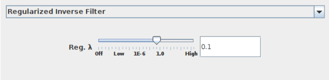
DeconvolutionLab2: Regularized Inverse Filter (RIF)
RIF a simple deconvolution approach, which involves coefficient-wise division in the Fourier domain (see Sage et al. 2017 for detail). To penalize noise amplification, RIF involves a regularization parameter $\lambda$:
D. Sage, L. Donati, F. Soulez, D. Fortun, G. Schmit, A. Seitz, R. Guiet, C. Vonesch, and M. Unser, “Decon- volutionLab2: An open-source software for deconvolution microscopy,” Methods 115, 28–41 (2017).
Usage examples
Example 1
Deconvolve the previously stored cell image (Section 3.1) with the regularized inverse filter using $\lambda$ = 0.001:
import os
from DeconvTest.modules.deconvolution import deconvolution_lab_rif
deconvolution_lab_rif(imagej_path=imagej_path,
                      inputfile=os.getcwd() + '/code_examples/convolved_cell.tif',
                      psffile=os.getcwd() + '/code_examples/psf.tif',
                      regularization_lambda=0.001,
                      outputfile=os.getcwd() + '/code_examples/deconvolved_rif.tif')

cell = Cell(filename='code_examples/deconvolved_rif.tif')
cell.show_2d_projections()

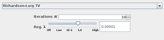
DeconvolutionLab2: Richardson-Lucy with Total Variance (RLTV)
RLTV is an iterative minimization approach, which -- similarly to RIF -- also involves regularization (see Sage et al. 2017 for detail). Thus, RLTV uses two parameters: the regularization $\lambda$ and the number of iterations:
D. Sage, L. Donati, F. Soulez, D. Fortun, G. Schmit, A. Seitz, R. Guiet, C. Vonesch, and M. Unser, “Decon- volutionLab2: An open-source software for deconvolution microscopy,” Methods 115, 28–41 (2017).
Usage examples
Example 1
Deconvolve the previously stored cell image (Section 3.1) with the Richardson-Lucy Total Variance algorithm using $\lambda$ = 0.001 and 5 iterations:
from DeconvTest.modules.deconvolution import deconvolution_lab_rltv
deconvolution_lab_rltv(imagej_path=imagej_path,
                       inputfile=os.getcwd() + '/code_examples/convolved_cell.tif',
                       psffile=os.getcwd() + '/code_examples/psf.tif',
                       rltv_lambda=0.001,
                       iterations=5,
                       outputfile=os.getcwd() + '/code_examples/deconvolved_rltv.tif')

cell = Cell(filename='code_examples/deconvolved_rltv.tif')
cell.show_2d_projections()

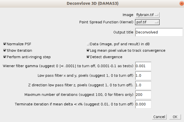
Iterative Deconvolve 3D (DAMAS)
DAMAS is an iterative deconvolution algorithm that includes multiple regularization techniques (see Dougherty et al. 2005 and the plugin documentation at http://www.optinav.info/Iterative-Deconvolve-3D.htm for details).
Six of the plugin's parameters can be adjusted from the DeconvTest framework:
- Normalize PSF (normalizes the PSF before deconvoltution)
- Detect divergence (stops the iteration if the changes in the image increase)
- Perform antiringing step (reduces artifacts from features close to the image border)
- Wiener filter $\gamma$ (regualization parameter)
- Low pass filter (regualization parameter)
- Terminate iteration if mean delta less than x% (stops the iteration if the changes in the image are less than the value of x)
R. Dougherty, “Extensions of DAMAS and Benefits and Limitations of Deconvolution in Beamforming,” (American Institute of Aeronautics and Astronautics, 2005).
Usage examples
Example 1
Deconvolve the previously stored cell image (Section 3.1) with the DAMAS algorithm using 2 iterations and the following parameters:
- Normalize PSF: False
- Detect divergence: False
- Perform antiringing step: True
- Wiener filter $\gamma$: 0.0001
- Low pass filter: 3
- Terminate iteration if mean $\delta$ <: 0.01
from DeconvTest.modules.deconvolution import iterative_deconvolve_3d
iterative_deconvolve_3d(imagej_path=imagej_path,
                        inputfile=os.getcwd() + '/code_examples/convolved_cell.tif',
                        psffile=os.getcwd() + '/code_examples/psf.tif',
                        outputfile=os.getcwd() + '/code_examples/deconvolved_iterative.tif',
                        normalize=False,
                        perform=False,
                        detect=True,
                        wiener=0.0001,
                        low=3,
                        terminate=0.01,
                        iterations=2)

cell = Cell(filename='code_examples/deconvolved_iterative.tif')
cell.show_2d_projections()

Quantification of deconvolution performance
After deconvolving synthetic images of cells, the performance of deconvolution can be quantified by comparing the images of reconstructed cells to the ground truth (initially generated cells) and computing the reconstruction errors. To quantify the reconstuction errors, the following two measures are computed:
- Root-mean-square error (RMSE):
where $x_i$ is the $i$-th pixel's value in the ground truth image, $y_i$ is the corresponding pixel value in the reconstructed image, and $N$ is the total number of pixels.
- Normalized root-mean-square error (NRMSE):
where $x_{max}$ and $x_{min}$ are the maximum and the minimum intensity values of the ground truth image, respectively.
cell = Cell(input_voxel_size=0.5,
            size=[10, 6, 6],
            phi=np.pi/4,
            theta=np.pi/2)
cell.show_2d_projections()
cell.save('code_examples/ground_truth_cell.tif')
psf = PSF(sigma=2,
          aspect_ratio=1.5)
cell.convolve(psf)
cell.show_2d_projections()


Compare the images of the cell before and after convolution:
gt_cell = Cell(filename='code_examples/ground_truth_cell.tif')
cell.compute_accuracy_measures(gt_cell)
Running DeconvTest in a batch mode
Simulation of microscopy experiments can be done in a batch mode, i.e. synthetic cells can be generated, convolved, deconvolved and quantified in a parallel manner. The number of processes that should be run in parallel is specified by the parameters max_threads. If the parameter print_progress is set to True, the progress of the computation and the remaining time will be printed out.
from DeconvTest import batch
batch.generate_cell_parameters(outputfile='code_examples/cell_parameters.csv',
                               number_of_cells=3,
                               size_mean_and_std=(10, 2),
                               equal_dimensions=False)
pd.read_csv('code_examples/cell_parameters.csv', sep='\t', index_col=0)
Generate the cells with voxel size 0.2 µm per px running 4 processes in parallel:
batch.generate_cells_batch(params_file='code_examples/cell_parameters.csv',
                           outputfolder='code_examples/input_cells',
                           input_voxel_size=0.2,
                           max_threads=4,
                           print_progress=True)
Cell images are saved in the specified directory together with their metadata, which is stored in a csv file:
sorted(os.listdir('code_examples/input_cells'))
pd.read_csv('code_examples/input_cells/cell_002.csv', sep='\t',
            index_col=0, header=None).transpose()
Generate 4 PSF images with resolution 0.2 µm per px and all combinations of given xy standard deviations and elongation:
batch.generate_psfs_batch(outputfolder='code_examples/psfs',
                          psf_sigmas=[0.3, 1],
                          psf_aspect_ratios=[1.5, 4],
                          input_voxel_size=[0.2],
                          max_threads=4,
                          print_progress=False)
PSF images are saved in the specified directory together with their metadata:
sorted(os.listdir('code_examples/psfs'))
Convolve all input cells with all PSFs:
batch.convolve_batch(inputfolder='code_examples/input_cells',
                     psffolder='code_examples/psfs',
                     outputfolder='code_examples/convolved',
                     max_threads=4,
                     print_progress=False)
For each PSF, a directory is generated where the convolved cells are stored. The PSF itself is also stored together with its metadata.
The output file structure is as follows:
- PSF 1 image
- PSF 1 metadata
- folder with convolution results for PSF 1
- cell 1 image
- cell 1 metadata
- cell 2 image
- cell 2 metadata
- ...
- PSF 2 image
- PSF 2 metadata
- folder with convolution results for PSF 2
- cell 1 image
- cell 1 metadata
- cell 2 image
- cell 2 metadata
- ...
- ...
sorted(os.listdir('code_examples/convolved'))
Each PSF directory contains convolution results for all input cells together with the metadata:
sorted(os.listdir('code_examples/convolved/psf_sigma_1_aspect_ratio_1.5'))
Resize the convolved cells to voxel sizes 0.5 µm in all axes, as well as 0.5 µm in xy and 1 µm in z:
batch.resize_batch(inputfolder='code_examples/convolved',
                   outputfolder='code_examples/resized',
                   voxel_sizes_for_resizing=[0.5, [1, 0.5, 0.5]],
                   max_threads=4,
                   print_progress=False)
For each combination of voxel size and PSF, a new directory was created. PSF images are also resized. The output file structure is as follows:
- PSF 1, resolution 1: image
- PSF 1, resolution 1: metadata
- folder with resizing results for PSF 1, resolution 1
- cell 1 image
- cell 1 metadata
- cell 2 image
- cell 2 metadata
- ...
- PSF 1, resolution 2: image
- PSF 1, resolution 2: metadata
- folder with resizing results for PSF 1, resolution 2
- cell 1 image
- cell 1 metadata
- cell 2 image
- cell 2 metadata
- ...
- PSF 2, resolution 1: image
- PSF 2, resolution 1: metadata
- folder with resizing results for PSF 2, resolution 1
- cell 1 image
- cell 1 metadata
- cell 2 image
- cell 2 metadata
- ...
- PSF 2, resolution 2: image
- PSF 2, resolution 2: metadata
- folder with resizing results for PSF 2, resolution 2
- cell 1 image
- cell 1 metadata
- cell 2 image
- cell 2 metadata
- ...
- ...
sorted(os.listdir('code_examples/resized'))
Each directory contains corresponding cells with the metadata:
sorted(os.listdir('code_examples/resized/psf_sigma_0.3_aspect_ratio_4_voxel_size_[1._0.5_0.5]'))
Add Gaussian noise with SNRs 5 and 10 to all resized cells:
batch.add_noise_batch(inputfolder='code_examples/resized',
                      outputfolder='code_examples/noise',
                      snr=[5, 10],
                      noise_kind='gaussian',
                      max_threads=4,
                      print_progress=False)
The output file structure is as follows:
- PSF 1, resoluton 1: image
- PSF 1, resoluton 1: metadata
- folder with convolution results for PSF 1, resoluton 1, SNR 1
- cell 1 image
- cell 1 metadata
- cell 2 image
- cell 2 metadata
- ...
- folder with convolution results for PSF 1, resoluton 1, SNR 2
- cell 1 image
- cell 1 metadata
- cell 2 image
- cell 2 metadata
- ...
- ...
- PSF 2, resoluton 2: image
- PSF 2, resoluton 2: metadata
- folder with convolution results for PSF 2, resoluton 2, SNR 1
- cell 1 image
- cell 1 metadata
- cell 2 image
- cell 2 metadata
- ...
- folder with convolution results for PSF 2, resoluton 2, SNR 2
- cell 1 image
- cell 1 metadata
- cell 2 image
- cell 2 metadata
- ...
- ...
sorted(os.listdir('code_examples/noise'))[0:10]
Example 2: generate multicellular samples
Generate parameters for samples with varying number of cells:
batch.generate_cell_parameters(outputfile='code_examples/stack_parameters.csv',
                               number_of_stacks=3,
                               number_of_cells=[3, 5],
                               size_mean_and_std=(10, 2),
                               equal_dimensions=False)
pd.read_csv('code_examples/stack_parameters.csv', sep='\t', index_col=0)
Generate multicellular samples with voxel size 2 µm per px in z and 0.5 µm per px in xy:
batch.generate_cells_batch(params_file='code_examples/stack_parameters.csv',
                           stack_size_microns=[60, 100, 100],
                           outputfolder='code_examples/input_stacks',
                           input_voxel_size=[2, 0.5, 0.5],
                           max_threads=4,
                           print_progress=False)
sorted(os.listdir('code_examples/input_stacks'))
Generate PSFs with voxel size 2 µm per px in z and 0.5 µm per px in xy, standard deviation 0.3 µm in xy and elongation 1.5:
batch.generate_psfs_batch(outputfolder='code_examples/psfs2',
                          psf_sigmas=[0.3],
                          psf_aspect_ratios=[1.5],
                          input_voxel_size=[2, 0.5, 0.5],
                          max_threads=4,
                          print_progress=False)
Convolve all input images with all PSFs:
batch.convolve_batch(inputfolder='code_examples/input_stacks',
                     psffolder='code_examples/psfs2',
                     outputfolder='code_examples/stacks_convolved',
                     max_threads=4,
                     print_progress=False)
Resize the convolved images:
batch.resize_batch(inputfolder='code_examples/stacks_convolved',
                   outputfolder='code_examples/stacks_resized',
                   voxel_sizes_for_resizing=[[3, 0.5, 0.5]],
                   max_threads=4,
                   print_progress=False)
Add Poisson noise to the resized images:
batch.add_noise_batch(inputfolder='code_examples/stacks_resized',
                      outputfolder='code_examples/stacks_noise',
                      snr=[2],
                      noise_kind='poisson',
                      max_threads=4,
                      print_progress=False)
Example 3: run the full simulation on single cell images
Generate cell parameters, cells, PSFs, convolve the cells with the PSFs and add noise:
batch.generate_cell_parameters(outputfile='code_examples/cell_parameters.csv',
                               number_of_cells=1,
                               size_mean_and_std=(8, 2),
                               equal_dimensions=False)
batch.generate_cells_batch(params_file='code_examples/cell_parameters.csv',
                           outputfolder='code_examples/input_cells_deconv',
                           input_voxel_size=0.3,
                           max_threads=4,
                           print_progress=False)
batch.generate_psfs_batch(outputfolder='code_examples/psfs_deconv',
                          psf_sigmas=[0.3], psf_aspect_ratios=[1.5],
                          input_voxel_size=[0.3],
                          max_threads=4,
                          print_progress=False)
batch.convolve_batch(inputfolder='code_examples/input_cells_deconv',
                     psffolder='code_examples/psfs_deconv',
                     outputfolder='code_examples/convolved_deconv',
                     max_threads=4,
                     print_progress=False)
batch.resize_batch(inputfolder='code_examples/convolved_deconv',
                  outputfolder='code_examples/resized_deconv',
                  voxel_sizes_for_resizing=[0.5],
                  max_threads=4,
                  print_progress=False)
batch.add_noise_batch(inputfolder='code_examples/resized_deconv',
                      outputfolder='code_examples/noise_deconv',
                      snr=[10],
                      noise_kind='poisson',
                      max_threads=4,
                      print_progress=False)
Deconvolve the generated cells with Regularize Inverse Filter and with Richardson-Lucy Total Variance algorithm, using two sets of parameters for each algorithm:
batch.deconvolve_batch(inputfolder='code_examples/noise_deconv/',
                      outputfolder='code_examples/deconvolved/',
                      deconvolution_algorithm=['deconvolution_lab_rif', 'deconvolution_lab_rltv'],
                      deconvolution_lab_rif_regularization_labmda=[0.001, 0.002],
                      deconvolution_lab_rltv_regularization_labmda=[0.0001],
                      deconvolution_lab_rltv_iterations=[10, 15],
                      print_progress=False,
                      max_threads=4)
os.listdir('code_examples/deconvolved/')
os.listdir('code_examples/deconvolved/deconvolution_lab_rif_regularization_labmda=0.001')
os.listdir('code_examples/deconvolved/deconvolution_lab_rif_regularization_labmda=0.001/psf_sigma_0.3_aspect_ratio_1.5_voxel_size_[0.5_0.5_0.5]_noise_poisson_snr=10')
Compare the deconvolved images to the ground truth:
batch.accuracy_batch(inputfolder='code_examples/deconvolved',
                     reffolder='code_examples/input_cells_deconv',
                     outputfolder='code_examples/accuracy',
                     max_threads=4,
                     print_progress=False)
All accuracy values are combined into a single csv file:
pd.read_csv('code_examples/accuracy.csv', sep='\t', index_col=0)
Running in silico deconvolution experiments with the "run_simulation" script
Specifying parameters of the experiment
An in silico microscopy and deconvolution experiment can be run via executing a specifically developed script, which accepts the parameters of the experiment specified in a csv config file.
The following are the parameters and their default values (if any) used by the script:
| Parameter | Description | Default value |
|---|---|---|
| simulation_folder | directory to save the simulation output | ./test_simulation |
| simulation_steps | list of simulation steps to run; valid values are: generate_cells, generate_psfs, convolve, resize, add_noise, deconvolve, accuracy |
['generate_cells', 'generate_psfs', 'convolve', 'resize', 'add_noise','deconvolve', 'accuracy'] |
| cell_parameter_filename | csv file name in the simulation_folder to save cell parameters |
cell_parameters.csv |
| inputfolder | directory in the simulation_folder to save generated synthetic cells |
input |
| psffolder | directory in the simulation_folder to save generated PSF images |
psf |
| convolve_results_folder | directory in the simulation_folder to save the results of convolution of input cells with PSFs |
convolved |
| resize_results_folder | directory in the simulation_folder to save the downsized images |
resized |
| add_noise_results_folder | directory in the simulation_folder to save images after adding noise |
noise |
| deconvolve_results_folder | directory in the simulation_folder to save deconvolved images |
deconvolved |
| accuracy_results_folder | directory in the simulation_folder to save the deconvolution performance results |
accuracy_measures |
| log_folder | directory in the simulation_folder to store computing time |
timelog |
| max_threads | the maximal number of processes to run in parallel | 4 |
| print_progress | if True, the progress of the computation will be printed | True |
| number_of_stacks | number of multicellular samples to generate; if None, no multicellular samples will be generated, but only single cells |
None |
| number_of_cells | number of single cells to generate or number of cells per each multicellular stack; if a range is indicated, and the number_of_stacks parameter is not None, a random number will be chosen from this range to set the number of cells in each individual multicellular sample |
2 |
| input_cell_kind | type the input cell to generate; valid values are: ellipsoid, spiky_cell |
ellipsoid |
| size_mean_and_std | mean value and standard deviation for the cell size in micrometers; the cell size is drawn randomly from a Gaussian distribution with the given mean and standard deviation. | (10, 2) |
| equal_dimensions | if True, input cells will be generated as spheres; if False, input cells will be generated as ellipsoids with sizes for all three axes chosen independently | False |
| spikiness_range | range for the fraction of cell surface area covered by spikes (if input_cell_kind is spiky_cell) |
|
| spike_size_range | range for the standard deviation for the spike amplitude relative to the cell radius (if input_cell_kind is spiky_cell) |
|
| spike_smoothness_range | range for the width of the Gaussian filter that is used to smooth the spikes (if input_cell_kind is spiky_cell) |
|
| input_voxel_size | voxel size in z, y and x used to generate the cell image; if one value is provided, the voxel size is assume to be equal along all axes. | 0.3 |
| stack_size_microns | dimensions of the multicellular image stack in micrometers | [10, 100, 100] |
| psf_sigmas | standard deviation(s) of the PSF in xy in micrometers; a PSF image will be generated for each combination of the provided values of psf_sigmas and psf_aspect_ratios |
[0.1, 0.5] |
| psf_aspect_ratios | PSF aspect ratios; a PSF image will be generated for each combination of the provided values of psf_sigmas and psf_aspect_ratios |
[3] |
| voxel_sizes_for_resizing | list of new voxel sizes to which the input images should be resized; each item of the list is a scalar (for the same voxels size along all axes) or sequence of scalars (voxel size in z, y and x) | [[1, 0.5, 0.5]] |
| noise_kind | type of noise to add; valid values are: poisson, gaussian; if several values are provided, all noise types will be added in the given order; if the same number of values are provided for noise_kind and snr and the test_snr_combinations parameter is False, only one corresponding SNR will be used for each noise kind; for test_snr_combinations equal True see description of the test_snr_combinations parameter |
[poisson] |
| snr | target signal-to-noise ratio (SNR) value(s); for each provided value, a new image will be generated; if several values for noise_kind are provided, and the same nuber of values are provided for snr, one corresponding SNR will be used for each noise kind (only if test_snr_combinations parameter is False, for test_snr_combinations equal True see description of the test_snr_combinations parameter) |
[None, 5] |
| test_snr_combinations | if True, and several values are provided for the noise_kind parameter and snr parameter, all combinations of given SNRs will be used for all provided noise types (e.g. if noise_kind is [poisson, gaussian] and snr is [5, 10], the following four noise features will be applied: Poisson noise with SNR 5 + Gaussian noise with SNR 5, Poisson noise with SNR 5 + Gaussian noise with SNR 10, Poisson noise with SNR 10 + Gaussian noise with SNR 5, Poisson noise with SNR 10 + Gaussian noise with SNR 10) |
False |
| deconvolution_algorithm | deconvolution algorithm(s) that will be applied to deconvolve the input images; if a sequence of algorithms is provided, all algorithms from the sequence will be applied | [deconvolution_lab_rif, deconvolution_lab_rltv] |
| log_computing_time | if True, computing time spent on deconvolution will be recorded and stored in the log_folder |
True |
| deconvolution_lab_rif_regularization_lambda | regularization parameter for the RIF algorithm; if a sequence is provided, all values from the sequence will be tested | [0.001, 1] |
| deconvolution_lab_rltv_regularization_lambda | regularization parameter for the RLTV algorithm; if a sequence is provided, all values from the sequence will be tested in combination with the iterations parameter |
0.001 |
| deconvolution_lab_rltv_iterations | number of iterations in the RLTV algorithm; if a sequence is provided, all values from the sequence will be tested in combination with the rltv_lambda parameter |
[2, 3] |
| iterative_deconvolve_3d_normalize | Normalize PSF parameter for the Iterative Deconvolve 3D plugin; if a sequence is provided, all values from the sequence will be tested in combination with other parameters |
|
| iterative_deconvolve_3d_perform | Perform anti-ringig step parameter for the Iterative Deconvolve 3D plugin; if a sequence is provided, all values from the sequence will be tested in combination with other parameters |
|
| iterative_deconvolve_3d_detect | Detect divergence parameter for the Iterative Deconvolve 3D plugin; if a sequence is provided, all values from the sequence will be tested in combination with other parameters |
|
| iterative_deconvolve_3d_wiener | Wiener filter gamma parameter for the Iterative Deconvolve 3D plugin; <0.0001 to turn off, 0.0001 - 0.1 as tests; if a sequence is provided, all values from the sequence will be tested in combination with other parameters |
|
| iterative_deconvolve_3d_low | Low pass filter parameter for the Iterative Deconvolve 3D plugin, pixels; the same value is used for low pass filter in xy and z; if a sequence is provided, all values from the sequence will be tested in combination with other parameters |
|
| iterative_deconvolve_3d_terminate | Terminate iteration if mean delta < x% parameter for the Iterative Deconvolve 3D plugin; 0 to turn off; if a sequence is provided, all values from the sequence will be tested in combination with other parameters |
The parameter file does not have to specify all parameter values, but only those that should be different from the default values. This is how an example parameter file may look like:
pd.read_csv('example_config_file.csv', sep='\t', index_col=0, header=None).squeeze()
Running the experiment with the "run_simulation" script
To run a deconvolution experiment with specified settings, the run_simulation.py scipt should be copied to the directory of choice, and the following command should be executed:
python run_simulation.py <settings_file>
After the simulation is completed, the computed accuracy will be summarized in a csv file named the same as the accuracy_results_folder specified in the config file.
Running DeconvTest with external synthetic data
DeconvTest can also be used with externally generated synthetic images.
Usage examples
Example 1
Generate synthetic images with the software of your choice. Here is an example how this can be done using the DeconvolutionLab2 plugin of Fiji:
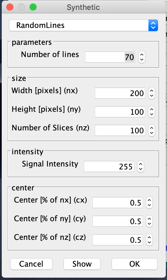
Generate synthetic PSF images. For instance, with DeconvolutionLab2 you can generate an Airy-disk-shaped PSF:
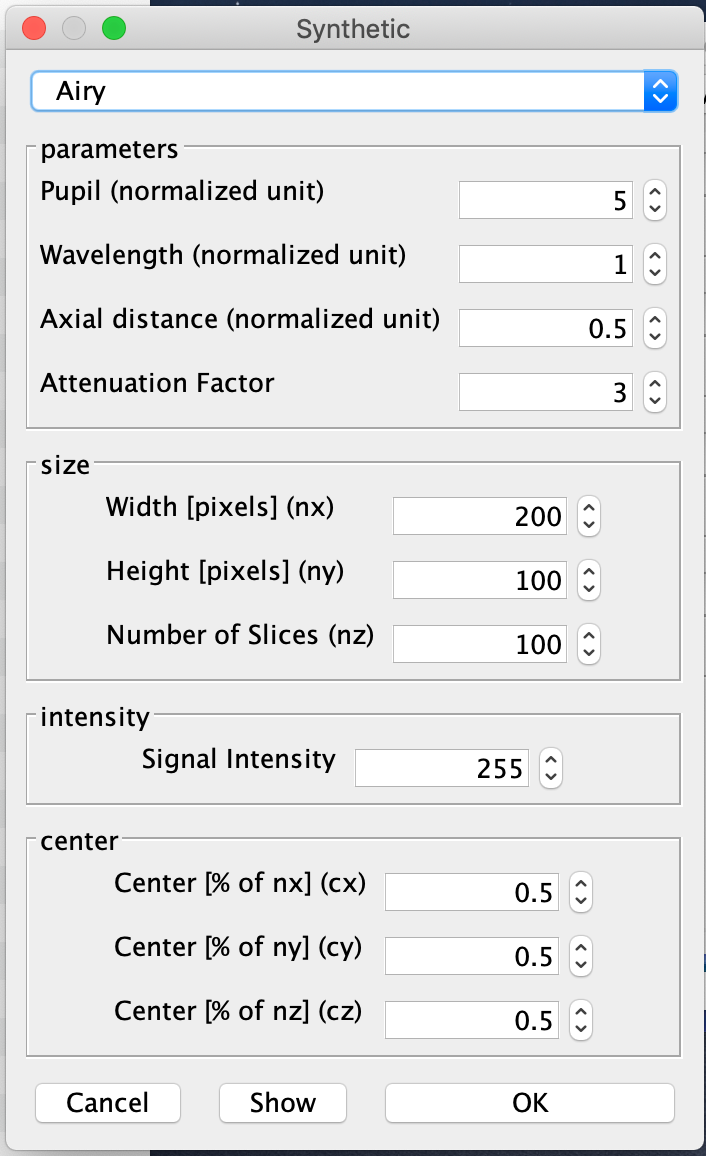
We generated two images with random lines and one airy-disk PSF and saved them in the folders 'data/synthetic/input/' and 'data/synthetic/psf/', respectively:
os.listdir('data/synthetic/input')
stack = Stack(filename='data/synthetic/input/RandomLines1.tif')
stack.show_2d_projections()

os.listdir('data/synthetic/psf')
psf = PSF(filename='data/synthetic/psf/psf_airy.tif')
psf.show_2d_projections()

As the next step, we need to create a metadata file with voxel size values for each image. Let's set voxel size to 1 µm in all dimensions:
from DeconvTest.classes.metadata import Metadata
for fn in os.listdir('data/synthetic/input/'):
    md = Metadata()
    md.set_voxel_size(1)
    md.to_csv('data/synthetic/input/' + fn[:-4] + '.csv', sep='\t', header=False)
For the PSF image, the size of the PSF needs to be stored in the metadata file. Since this value is only used to group the quantification results, any value can be provided. Moreover, isPSF parameter has to be set to True to indicate that we don't want to deconvolve this image during the deconvolution step.
for fn in os.listdir('data/synthetic/psf/'):
    md = Metadata()
    md.set_voxel_size(1)
    md['PSF sigma xy um'] = 1
    md['PSF aspect ratio'] = 1
    md['isPSF'] = 1
    md.to_csv('data/synthetic/psf/' + fn[:-4] + '.csv', sep='\t', header=False)
This is how the resulting metadata file looks like:
pd.read_csv('data/synthetic/psf/psf_airy.csv', sep='\t', index_col=0, header=None).squeeze()
Now, let's generate a configuration file to run DeconvTest workflow with these images. We will convolve the synthetic images and the PSF, add Poisson noise with SNR=5 and deconvolve the resulting data with two different values of the RIF $\lambda$:
config = pd.Series({'simulation_folder': 'data/synthetic/',
                    'simulation_steps': ['convolve', 'add_noise','deconvolve', 'accuracy'],
                    'max_threads': 1,
                    'noise_kind': ['poisson'],
                    'snr': [5],
                    'test_snr_combinations': False,
                    'deconvolution_algorithm': ['deconvolution_lab_rif'],
                    'deconvolution_lab_rif_regularization_lambda': [0.001, 1]
                    })
config.to_csv('config_external_data.csv', sep='\t', header=False)
config
Next, we run DeconvTest using this configuration file:
%run run_simulation.py config_external_data.csv
Let's now look at the resulting accuracy measures and plot the NRMSE depending on the value of RIF $\lambda$:
accuracy = pd.read_csv('data/synthetic/accuracy_measures.csv', sep='\t')
accuracy
import seaborn as sns
sns.swarmplot(data=accuracy, x='regularization_lambda', y='NRMSE')

It seems like the RIF $\lambda$ value of 1 worked much better for these data than the value of 0.001.
Running DeconvTest with external deconvolution results
Synthetic microscopy images generated with DeconvTest can be deconvolved using external software and evaluated for deconvolution errors using DeconvTest.
Usage examples
Example 1
First, we need to create a configuration file to generate synthetic images. Let's generate two ellipsoidal cells, convolve them with PSF, downsample, and add Poisson noise of SNR 5:
config = pd.Series({'simulation_folder': 'data/ext_deconvolution/',
                    'simulation_steps': ['generate_cells', 'generate_psfs', 'convolve', 'resize', 'add_noise'],
                    'max_threads': 1,
                    'number_of_cells': 2,
                    'input_cell_kind': 'ellipsoid',
                    'input_voxel_size': 0.3,
                    'psf_sigmas': [0.5],
                    'psf_aspect_ratios': [4],
                    'voxel_sizes_for_resizing': [0.5],
                    'noise_kind': ['poisson'],
                    'snr': [5]
                    })
config.to_csv('config_external_deconv.csv', sep='\t', header=False)
config
%run run_simulation.py config_external_deconv.csv
This resulted in generating two synthetic microscopy images and corresponding PSFs:
os.listdir('data/ext_deconvolution/noise')
os.listdir('data/ext_deconvolution/noise/psf_sigma_0.5_aspect_ratio_4.0_voxel_size_[0.5_0.5_0.5]_noise_poisson_snr=5.0')
psf = Stack(filename='data/ext_deconvolution/noise/psf_sigma_0.5_aspect_ratio_4.0_voxel_size_[0.5_0.5_0.5]_noise_poisson_snr=5.0/cell_001.tif')
psf.show_2d_projections()

psf = PSF(filename='data/ext_deconvolution/noise/psf_sigma_0.5_aspect_ratio_4.0_voxel_size_[0.5_0.5_0.5].tif')
psf.show_2d_projections()

As the next step, the generated images can be deconvolved with external software. For instance, here we deconvolved them with the Landweber algorithm from DeconvolutionLab2, which is not yet integrated into DeconvTest:
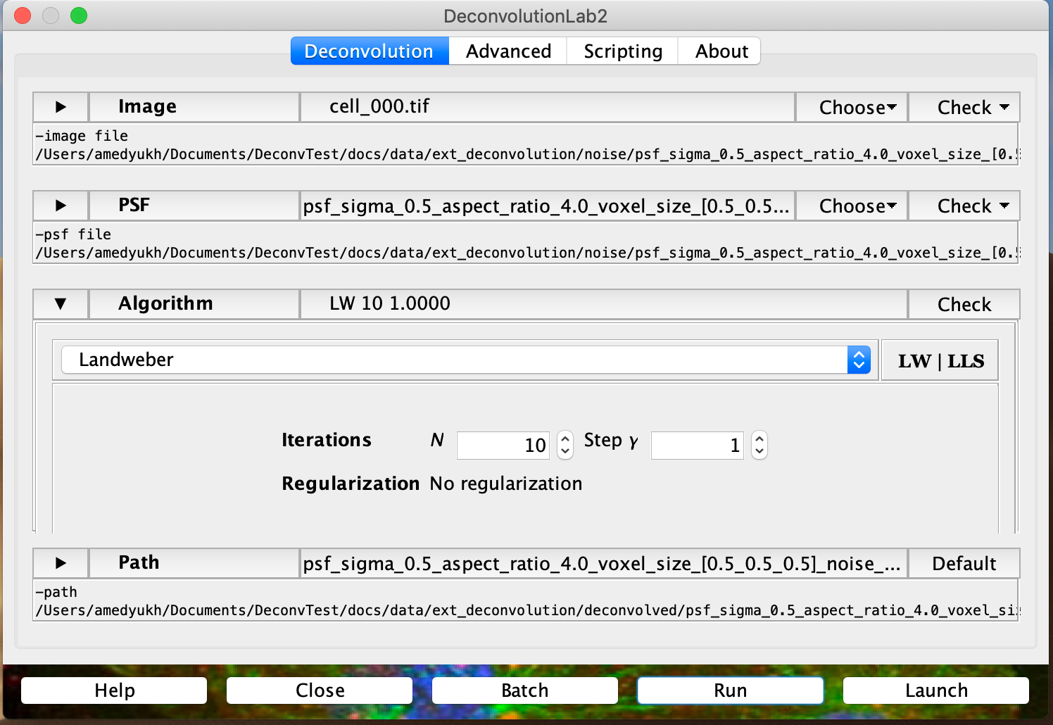
The user should make sure that the structure of the deconvolution output corresponds to the structure generated by a DeconvTest workflow. Thus, deconvolution results from each parameter combination should be kept in a separate folder (here we applied two different values of the parameter $\gamma$):
os.listdir('data/ext_deconvolution/deconvolved')
Each of these folders should contain a subfolder for each PSF/noise combination with the same naming as used before deconvolution:
os.listdir('data/ext_deconvolution/deconvolved/Landweber_gamma=1')
The subfolders contain the deconvolved images along with their metadata files:
os.listdir('data/ext_deconvolution/deconvolved/Landweber_gamma=1/psf_sigma_0.5_aspect_ratio_4.0_voxel_size_[0.5_0.5_0.5]_noise_poisson_snr=5.0')
The metadata files can be generated by copying the corresponding files before deconvolution and adding the values of the deconvolution parameters (in this case, Landweber gamma):
pd.read_csv('data/ext_deconvolution/deconvolved/Landweber_gamma=1/psf_sigma_0.5_aspect_ratio_4.0_voxel_size_[0.5_0.5_0.5]_noise_poisson_snr=5.0/cell_000.csv', sep='\t', index_col=0, header=None).squeeze()
Once this is done, we can specify another configuration file for running the quantification step of DeconvTest:
config = pd.Series({'simulation_folder': 'data/ext_deconvolution/',
                    'simulation_steps': ['accuracy'],
                    'max_threads': 1,
                    'inputfolder': 'deconvolved',
                    'reffolder': 'input'
                    })
config.to_csv('config_external_deconv_accuracy.csv', sep='\t', header=False)
config
%run run_simulation.py config_external_deconv_accuracy.csv
Let's now look at the resulting accuracy measures and plot the NRMSE depending on the value of Landweber $\gamma$ :
accuracy = pd.read_csv('data/ext_deconvolution/accuracy_measures.csv', sep='\t')
accuracy
import seaborn as sns
sns.swarmplot(data=accuracy, x='LW gamma', y='NRMSE')

Deconvolving microscopy images with the help of DeconvTest
Importantly, DeconvTest can help to deconvolve real microscopy images by identifying the optimal deconvolution parameters. For this, we first need to identify the properties of our microscopy images such as voxel size, PSF size, noise SNR, and the size of the features of interest. We then generate synthetic data with the same properties and deconvolve them with different settings using DeconvTest, which allows us to identify the deconvolution settings that result in the lowest errors. Finally, we can apply the identified algorithm and settings to reconstruct real microscopy images either within DeconvTest or using other software.
Identifying image properties
Thus, as the first step, we need to determine important image properties. Many of these can be identified using ImageJ.
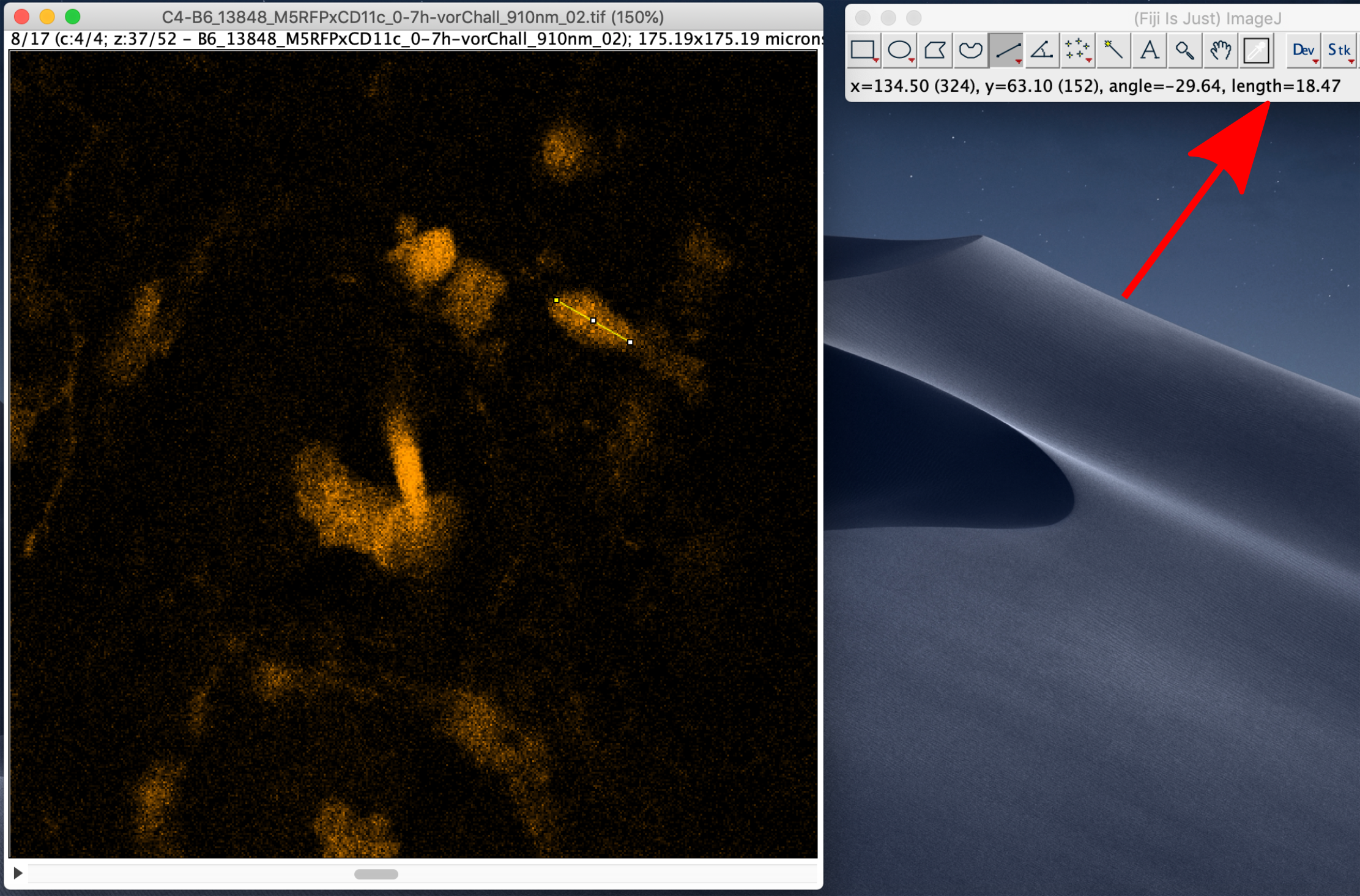
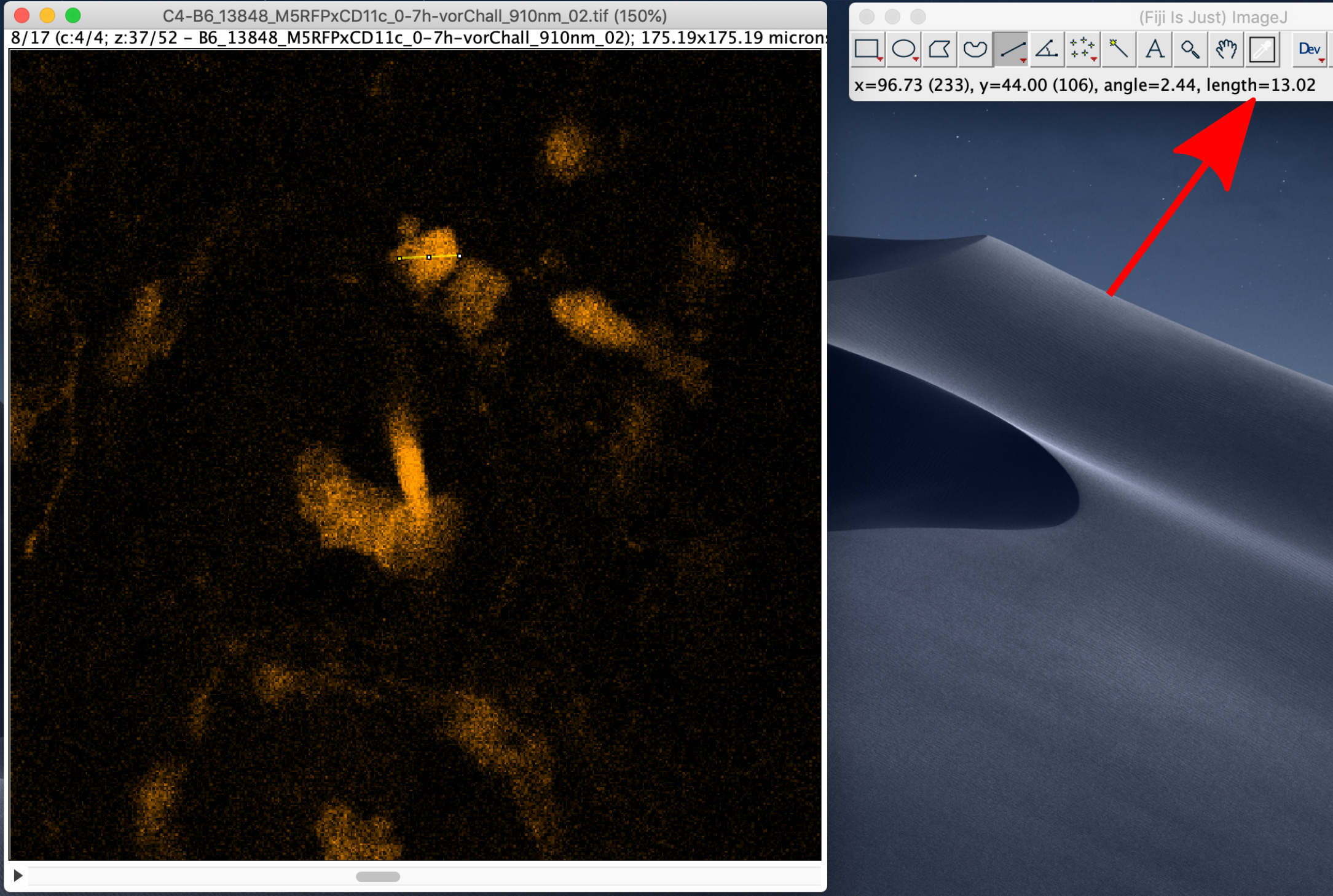
Size of the features of interest
To measure the size of the features of interest, e.g. cells, select the line tool and measure the size of a few objects. The length of the line will be displayed on the main panel of ImageJ using the same units that are set in the Image Properties:
Signal-to-noise ratio
To measure the signal-to-noise ratio (SNR), run Analyze -> Set Measurements and select Standard deviation and Mean gray value to be computed.
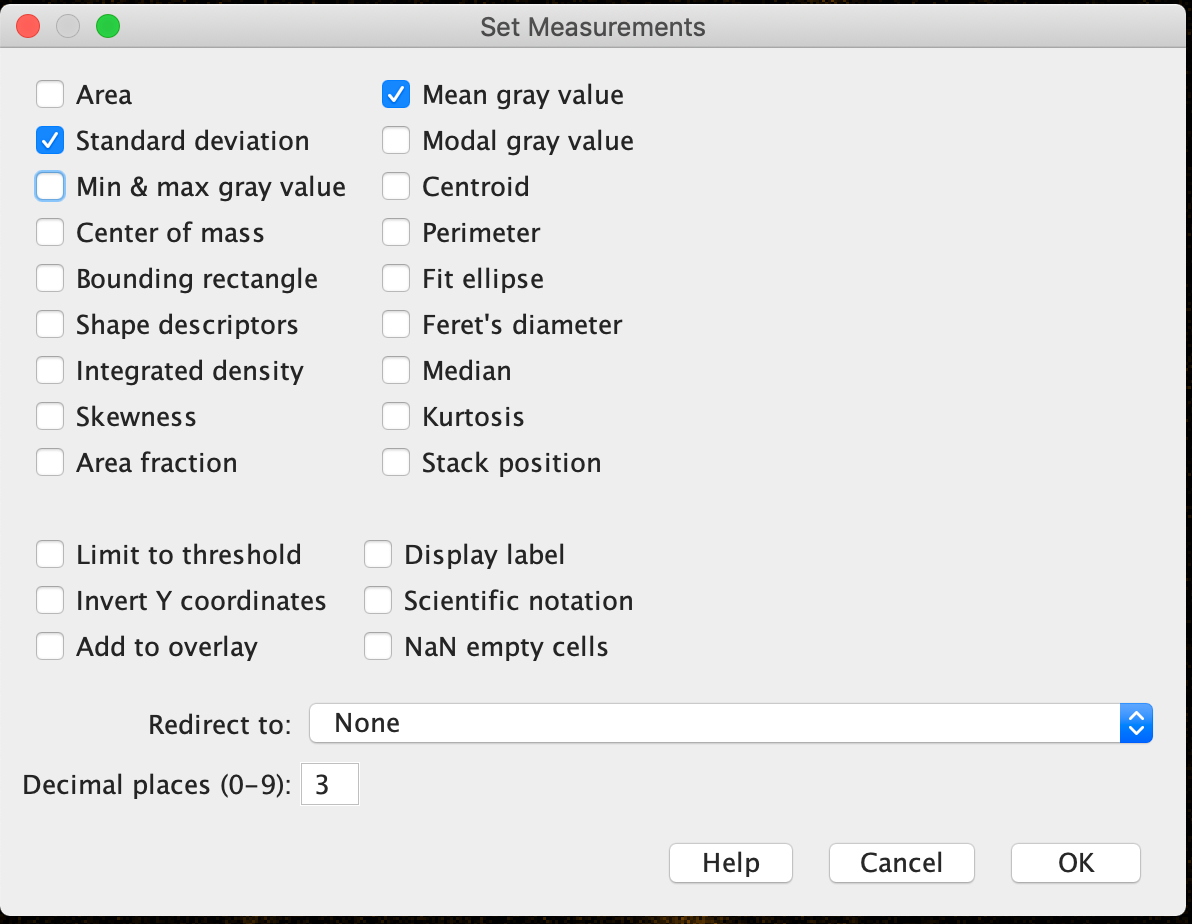
After that, select a few regions (e.g. with the elliptical selection tool) that are relatively bright but not over-saturated and run Analyze -> Measure.
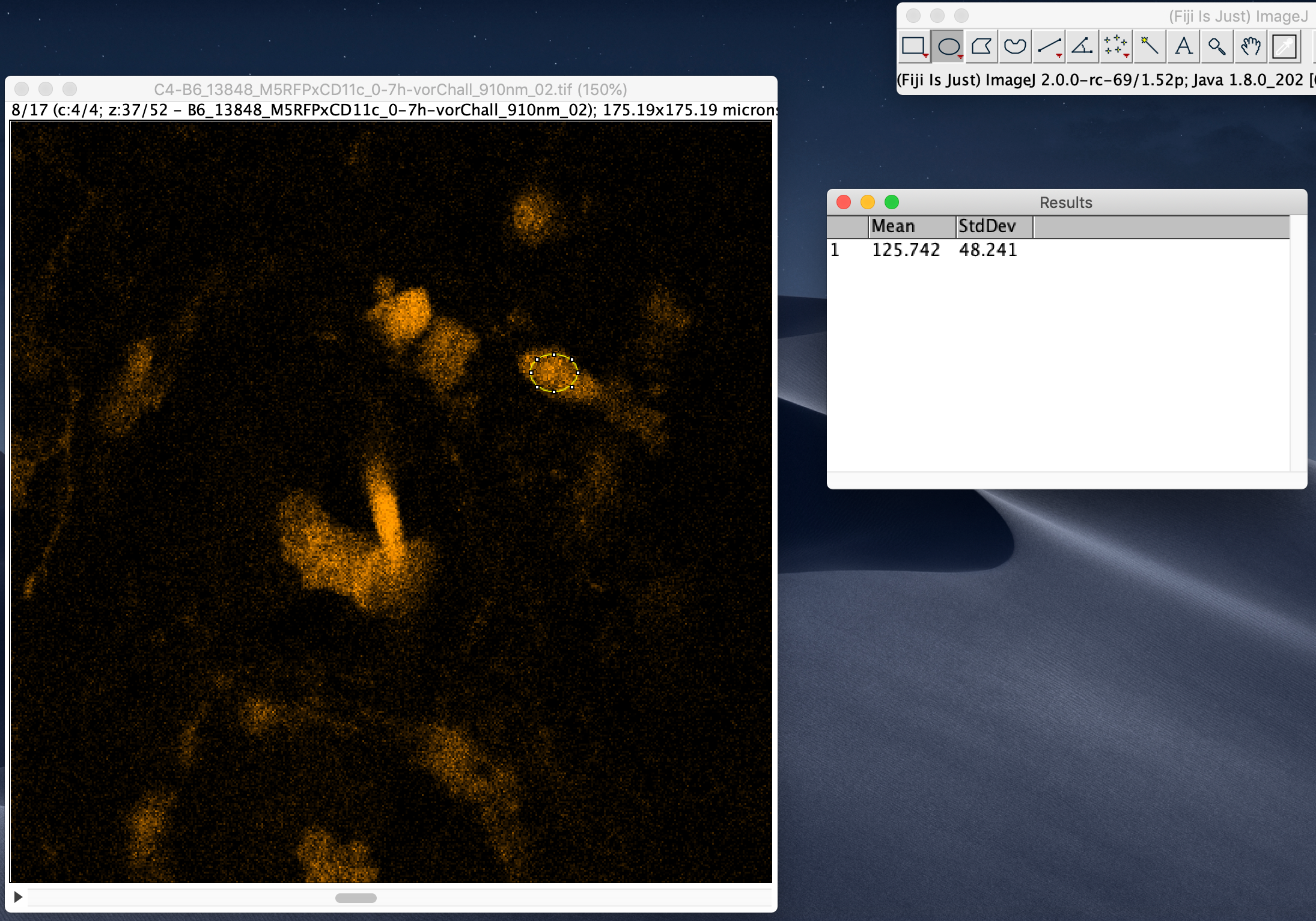
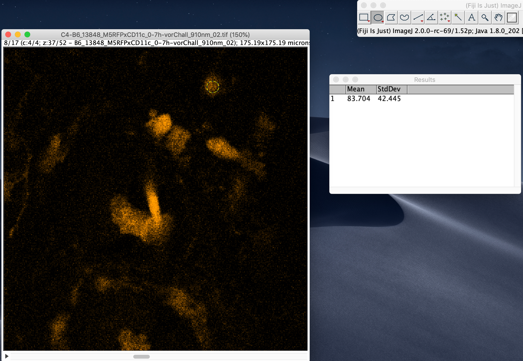
Divide the computed Mean gray value by the standard deviation to estimate SNR for each region. Take the smallest value for a conservative estimate.
Size of the point spread function
To estimate the size of the PSF, we need a PSF image, which can be either generated theoretically (e.g. using Huygens or ImageJ/Fiji) or measured by imaging fluorescent beads.
psf = PSF(filename='data/microscopy/real_data/psf_measured.tif')
psf.show_2d_projections()

DeconvTest provides tools to measure the size of the PSF by approximating is with a Gaussian function:
sigmas = psf.measure_psf_sigma()
sigmas
The measured values are in pixels and need to be multiplied by the corresponding voxel size to obtain the values in micrometers:
sigmas = sigmas * np.array([3, 0.415, 0.415])
sigmas
The aspect ratio of the PSF can be computed by dividing the standard deviation in z (the first value) by the standard deviation in x or y (the second or third value):
aspect = sigmas[0] / sigmas[1]
aspect
Running DeconvTest workflow with identified image properties
Now, when the microscopy image properties have been identified, we can adjust the DeconvTest configuration file to generate synthetic images with the same properties and deconvolve them with desired algorithms and parameters:
config = pd.Series({'simulation_folder': 'data/microscopy/',
                    'simulation_steps': ['generate_cells', 'generate_psfs',
                                         'convolve', 'resize', 'add_noise', 'deconvolve', 'accuracy'],
                    'max_threads': 1,
                    'number_of_cells': 10,
                    'size_mean_and_std': (15, 3),
                    'input_voxel_size': 0.1,
                    'psf_sigmas': 1.4,
                    'psf_aspect_ratios': 4,
                    'voxel_sizes_for_resizing': [[3, 0.45, 0.45]],
                    'noise_kind': ['poisson'],
                    'snr': 2,
                    'deconvolution_algorithm': ['deconvolution_lab_rif',
                                                'deconvolution_lab_rltv', 'iterative_deconvolve_3d'],
                    'deconvolution_lab_rif_regularization_lambda': [0.01, 0.1, 1, 10, 100, 1000],
                    'deconvolution_lab_rltv_regularization_lambda': [0.001, 0.01, 0.05, 0.1],
                    'deconvolution_lab_rltv_iterations': 5,
                    'iterative_deconvolve_3d_detect': 'FALSE',
                    'iterative_deconvolve_3d_low': [0, 2, 4, 6],
                    'iterative_deconvolve_3d_normalize': 'TRUE',
                    'iterative_deconvolve_3d_perform': 'TRUE',
                    'iterative_deconvolve_3d_terminate': 0.1,
                    'iterative_deconvolve_3d_wiener': [0, 0.1, 1.0, 10]
                    })
config.to_csv('config_microscopy_data.csv', sep='\t', header=False)
config
After running python run_simulation.py config_microscopy_data.csv, DeconvTest will generate a csv table with NRMSE values for all applied algorithms and parameter combinations:
accuracy = pd.read_csv('data/microscopy/accuracy_measures.csv', sep='\t')
accuracy[:10]
Here, the NRMSE values are provided per cell. To obtain average performance, we need to average among all deconvolved cells.
First, let's extract the algorithm name and the settings from the file name:
for i in range(len(accuracy)):
        setting = accuracy.iloc[i]['Name'].split('/')[-3]
        accuracy.at[i, 'Settings'] = setting
Then, we group by the extracted settings, compute the mean value and sort by NRMSE:
accuracy_summary = accuracy.groupby(['Settings']).mean().reset_index().sort_values('NRMSE')
accuracy_summary[:10]
The first line in the table now corresponds to the optimal deconvolution settings:
accuracy_summary.iloc[0]
Thus, DAMAS was identified as the optimal algorithm.
For the following parameters, only one value was tested:
- Normalize PSF: True
- Detect divergence: False
- Perform antiringing step: True
- Terminate iteration: 0.1
But for the other two parameters, the following values were identified as optimal:
- Wiener filter $\gamma$: 1
- Low pass filter: 2
Deconvolving microscopy images with identified optimal settings
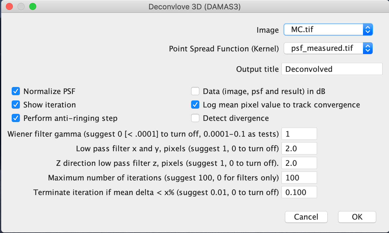
Using external deconvolution software
The real microscopy image can now be deconvolved with identified optimal settings. This can be done directly with the corresponding Fiji plugin by choosing the optimal parameter values. Make sure that the specified input and psf image have the same voxel size:
Using DeconvTest
Alternatively, the user can deconvolve images from within DeconvTest. For this, the images have to be stored in a subfolder that has the same name as the corresponding PSF image:
os.listdir('data/microscopy/real_data')
os.listdir('data/microscopy/real_data/psf_measured')
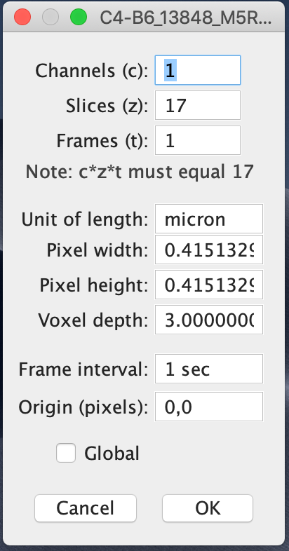
Image metadata must contain the voxel size values:
pd.read_csv('data/microscopy/real_data/psf_measured/MC.csv', sep='\t', index_col=0, header=None).squeeze()
pd.read_csv('data/microscopy/real_data/psf_measured.csv', sep='\t', index_col=0, header=None).squeeze()
Next, we need to specify a configuration file to run deconvolution and run the DeconvTest workflow with it:
config = pd.Series({'simulation_folder': 'data/microscopy/',
                    'simulation_steps': ['deconvolve'],
                    'inputfolder': 'real_data',
                    'deconvolve_results_folder': 'real_deconvolved',
                    'max_threads': 1,
                    'deconvolution_algorithm': ['iterative_deconvolve_3d'],
                    'iterative_deconvolve_3d_detect': 'FALSE',
                    'iterative_deconvolve_3d_low': 2,
                    'iterative_deconvolve_3d_normalize': 'TRUE',
                    'iterative_deconvolve_3d_perform': 'TRUE',
                    'iterative_deconvolve_3d_terminate': 0.1,
                    'iterative_deconvolve_3d_wiener': 1
                    })
config.to_csv('config_microscopy_data_deconvolve.csv', sep='\t', header=False)
config